2.6.1 Landau-Lifshitz-Gilbert equation with Slonczewski
spin-transfer torque term
In order to introduce a model equation for magnetization dynamics
in presence of spin polarized currents, let us first consider the
model derived by Slonczewski in Ref. [44]. In
his paper, a five layers structure is considered. In this
structure, the first, the third and the fifth layers are
constituted by paramagnetic conductors and the second and the
fourth layers are ferromagnetic conductors (it is a three layers
structure as the one mentioned in the introduction with
paramagnetic conductors as spacer and contacts). The multilayers
system is traversed by electric current normal to the layers
plane. The electron spins, polarized by the fixed ferromagnetic
layer (the second layer) are injected by passing through the
paramagnetic spacer into the free ferromagnetic layer (the forth
layer) where the interaction between spin polarized current and
magnetization takes place. The magnetic state of the ferromagnetic
layers is described by two vectors
and
representing macroscopic (total) spin orientation
per unit area of the fixed and the free ferromagnetic layers,
respectively. The connection of this two vectors with the total
spin momenta
and
(which have the
dimension of angular momenta) is given by the equations
,
, where is the cross-sectional area of the
multilayers structure. By using a semiclassical approach to treat
spin transfer between the two ferromagnetic layers, Slonczewski
derived the following generalized LLG equation (see Eq.(15)
in [44]):
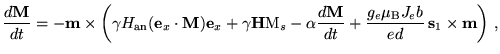
(2.74)
where
,
are the unit-vectors along
,
, is the absolute value of
the gyromagnetic ratio, is the anisotropy field constant,
is the unit vector along the anisotropy axis
(in-plane anisotropy), the Gilbert damping constant,
the current density (electric current per unit surface),
is the absolute value of the electron charge, a scalar
function given by the following expression
(2.75)
and is the spin polarizing factor of the incident current
which gives the percent amount of electrons that are polarized in
the
direction (see Ref. [44] for
details). The current in Eq. (2.74) is assumed
to be positive when the charges move from the fixed to the free
layer. Let us notice that in Eq. (2.74) the
ferromagnetic body is assumed to be uniaxial with anisotropy axis
along
. In the sequel, we will remove this simplifying
assumption by taking into account the effect of the strong
demagnetizing field normal to the plane of the layer in order to
consider the thin-film geometrical nature of the free layer. Our
next purpose is to derive from Eq. (2.74) an
equation for magnetization dynamics. We will carry out this
derivation by using slightly different notation and translating
all the quantities in practical MKSA units.
First of all, let us introduce a system of cartesian unit vectors
,
, where
is normal to the film plane and pointing in the
direction of the fixed layer, and
is along the
in-plane easy axis (in the Slonczewski notation
). The current density will be denoted by
(instead of as in Eq. (2.74)), the
anisotropy field as
an and the function
in Eq. (2.75) will be denoted with to
avoid confusion with the free energy and the Landé factor
that will be used in the following. In this reference frame the
current density vector is
, which means
that when the electrons travel in the direction opposite
to
, namely from the fixed to the free layer.
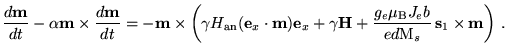
By using these modified notations and by including the effects of
the demagnetizing field
and the applied field
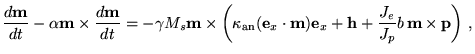
, Eq. (2.74) becomes
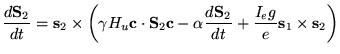
(2.76)
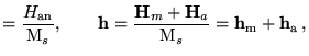
where
S. The sum of the demagnetizing
field
and the applied field
will be
indicated in he following by
to shorten the notation,
i.e.
(2.77)
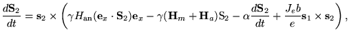
In order to check the correctness of the signs of precessional
terms in Eq. (2.76), let us transform this
equation in a slightly different form, by factoring out from the
parenthesis the constant
S. For the sake of simplicity,
we will carry out this derivation in the case and
. We have then the following equation
(2.78)
We observe now that what is generally defined as effective
anisotropy field is given by
anan
(2.79)
The minus sign in this equation is due to the fact that the
direction of
is opposite to the direction of
magnetization. This issue will be discussed below. By substituting
Eq. (2.79) into
Eq. (2.78) we obtain
(2.80)
where
effanan
(2.81)
Equation (2.80) is the correct precession
equation for the spin vector dynamics.
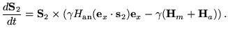
Next, we want to derive the dynamical equation for the
magnetization vector
associated with the free layer.
In this respect, we have first to consider the relation between
and
. The total magnetic moment
associated with the free layer is given by
(2.82)
where has been introduced above and coincides with the area of
the surface of the film. The magnetization
is
obtained by dividing the total magnetic moment by the volume of
the film V:
(2.83)
where is the free layer thickness, thus we obtain the
following relations
(2.84)
where is the Landè factor for electrons,
B is
the Bhor magneton, and the relation
B has been used. Let us notice that, as a consequence of
Eq. (2.84), we have
(2.85)
where
M is the saturation magnetization
and
is the unit vector along
. By multiplying
both sides of Eq. (2.76) by the factor
and taking into account
Eq. (2.85), one ends up with the following equation
(2.86)
which can be further normalized by dividing both sides by
M, leading to
(2.87)
In order to derive a time normalized form of the equation, we
factor out from the parenthesis the term
which has
the dimension of a frequency, and thus we have
(2.88)
where
an
(2.89)
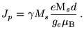
where
aa,
m. Finally, let us denote the
direction of magnetization in the fixed layer by
.
According to the previous reasoning, this direction is opposite to
, i.e.
. We also define the
following constant which has the physical dimension of a current
density:
(2.90)
By using the notations defined above, we arrive to the following
form of Eq. (2.88):
(2.91)
where the scalar (and dimensionless) function , in the new
notations, is
(2.92)
By measuring the time in units of
, and
introducing the following definitions,
(2.93)
equation (2.91) can be written in the compact form
(2.94)
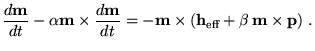
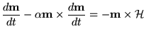
In the following, we will find convenient to recast LLG equation
in the following compact form:
eff
(2.95)
where
eff
(2.96)
Equation (2.95) is formally identical to LLG when
there are no current-driven torque term. With the definition of
the generalized effective field
eff we included
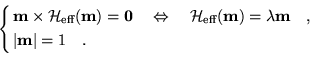
the current-driven torque inside the effective field. The
micromagnetic equilibria including spin torque effect are now
related to the following equations similar to
Eqs. (2.22):
The basic difference between the ordinary effective field
and the generalized effective field
is that the first one can be derived by the
gradient of a free energy, while the second one cannot.
Next:2.6.2 Discussion about units Up:2.6 LLG dynamics driven Previous:2.6 LLG dynamics drivenContents
Massimiliano d'Aquino
2005-11-26

![$\displaystyle g(\textbf{s}_1 \cdot \textbf{s}_2)=\left[ -4 +(1+P)^3 \frac{(3+ \textbf{s}_1 \cdot \textbf{s}_2 )}{4P^{3/2}} \right]^{-1}$](img784.gif)

![$\displaystyle b=b(\textbf{{m}})=\left[ -4 +(1+P)^3 \frac{(3+ \textbf{{m}}\cdot \textbf{p} )}{4P^{3/2}} \right]^{-1} .$](img831.gif)
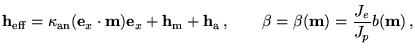
 eff
eff