2.6.3.1 Perturbative technique

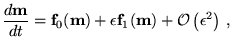
In order to establish the existence, the number, the stability and the locations of these limit cycles we can exploit the fact that both $\alpha$ and $\beta$ are small quantities (in the order of $10^{-2}\div 10^{-3}$). Thus, we can study the dynamics under the influence of spin-injection as perturbation of the case $\alpha=0$, $\beta=0$. To this end, we introduce the perturbation parameter $\epsilon$ such that $\alpha= \alpha_0 \epsilon , \beta= \beta_0 \epsilon$, and write Eq.(2.105) in the following perturbative form

$$\frac{d \textbf{{m}}}{d t}= \textbf{f}_0(\textbf{{m}}) +\epsilon \textbf{f}_1(\textbf{{m}}) + {\mathcal{O}}\left( \epsilon^2 \right) ,$$ (2.109)

where

$$\textbf{f}_0(\textbf{{m}}) = -\textbf{{m}}\times \textbf{h}_{\text{eff}}$$ (2.110)

$$\textbf{f}_1(\textbf{{m}}) = -{\beta_0}\textbf{{m}}\times \left( \textbf{{m}}\times \textbf... ...bf{{m}}\times \left( \textbf{{m}}\times \textbf{h}_{\text{eff}} \right) \quad.$$ (2.111)

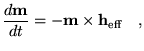
The unperturbed dynamics described by the undamped LLG

$$\frac{d\textbf{{m}}}{dt}=-\textbf{{m}}\times \textbf{h}_{\text{eff}}\quad,$$ (2.112)

can be treated analytically [50], for any constant applied field, by using the fact that conservative dynamics admits two integrals of motions (section 1.3.5):

$$m_x^2 + m_y^2 + m_z^2 = 1$$ (2.113)

$$g(\textbf{{m}})=g_0 \quad,$$ (2.114)

where $g_0$ is a constant depending on initial conditions. Similarly to the analysis performed in section 2.5, we will denote the trajectory of the unperturbed LLG equation, corresponding to the value $g_0$, with the notation $\textbf{{m}}_{g_0}(t)$ and the corresponding period with $T_{g_0}$. These trajectories are all closed and periodic (except separatrices which begin and finish at saddles equilibria). When the perturbation term $\epsilon \textbf{f}_1(\textbf{{m}})$ is introduced, almost all closed trajectories are slightly modified and collectively form spiral-shaped trajectories toward attractors. There are only special trajectories which remain (at first order in $\epsilon$) practically unchanged and become limit cycles of the perturbed system, provided that $\epsilon$ is small enough. In addition, each limit cycle is $\epsilon$-close to the conservative trajectory from which it has been generated. 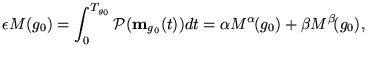The value of energy of the unperturbed special trajectories which generate limit cycles can be found from the zeros of the Melnikov function (see Appendix and Ref. [43]):

$$M(g_0)=\int_0^{T_{g_0}} \textbf{{m}}_{g_0}(t) \cdot \left[\textb... ...xtbf{{m}}_{g_0}(t)) \times \textbf{f}_1(\textbf{{m}}_{g_0}(t)) \right] dt .$$ (2.115)

In our case, by using straightforward algebra, one can prove that the function $M(g_0)$ can be expressed as:

$$\epsilon M(g_0)=\int_0^{T_{g_0}} {\mathcal{P}}(\textbf{{m}}_{g_0}(t)) dt = \alpha M^\alpha\! (g_0) + \beta M^\beta\!(g_0),$$ (2.116)

where $\alpha M^\alpha\!(g_0)$ and $\beta M^\beta\!(g_0)$ respectively correspond to the integral over one period of the first and second terms at the right hand side of Eq. (2.107). The expression (2.116) of the $M(g_0)$ provides also a physical justification of the method: the existence of limit cycles requires an average balance between loss and gain of energy. We observe that this result is analogous to the one discussed in section 2.5.