We now introduce a spatially discretized version of the
mathematical model. The discussion presented below is considerably
general and thus applicable to all the usual spatial
discretization techniques [52].
To start the discussion, let us assume that the magnetic body has
been subdivided in cells or finite elements. We denote the
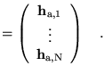
magnetization vector associated to the -th cell or node by
. Analogously, the effective and the
applied fields at each cell will be denoted by the vector
,
. In addition to the
cell-vectors, we introduce another notation for the mesh vectors
which include the information of all cells of the mesh. In this
respect, we will indicate with
,
eff,
a the vectors in
given by:

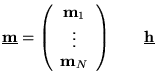 eff
eff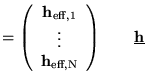 a
a