Thus, to summarize the previously derived results, we can write
the expression for the first-order variation of the free energy
functional (1.53):
(1.64)
Now we claim the fact that the variation
has to
satisfy the constraint
. For this reason,
it can be easily observed that the most general variation is a
rotation of the vector field
, that is
(1.65)
where the vector
represents an elementary
rotation of angle
. By substituting this expression
in Eq. (1.64) and remembering that
,
one obtains:
(1.66)
Since the elementary rotation
is arbitrary,
Eq. (1.66) can be identically zero if and
only if:
In the second equation the fact that
implies that
, as
the vectors
and
are always
orthogonal; in fact, the only way their vector product can vanish
is that
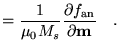
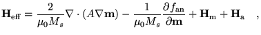
is identically zero. We introduce now
the effective field
(1.68)
where the first two terms take into account the exchange and
anisotropy interjections. In other words, these interactions
effectively act on the magnetization as they were suitable fields:
The Brown's equations allow one to find the equilibrium
configuration of the magnetization within the body. The first
equation states that the torque exerted on magnetization by the
effective field must vanish at the equilibrium. It is important to
notice that Eqs. (1.71) are nonlinear, since the
effective field (1.68) has a functional
dependance on the whole vector field
. As we will
discuss later, the existence of exact analytical solutions is
subject to appropriate simplifying assumptions. For this reason,
in most cases numerical solution of Eqs. (1.71) is
required. In addition, as mentioned in
section 1.1.2, the model must be completed with a
dynamic equation to properly describe the evolution of the system.
This will be done in the following section.
Next:1.3 The Dynamic Equation Up:1.2 Micromagnetic Equilibrium Previous:1.2.1.4 Zeeman energyContents
Massimiliano d'Aquino
2005-11-26

![\begin{displaymath}\begin{split}
\delta G=-\int_\Omega \left[ 2\nabla\cdot(A\na...
...{n}}\cdot\delta \textbf{{m}}\right] dS =0 \quad.
\end{split}\end{displaymath}](img395.gif)
![\begin{displaymath}\begin{split}
\delta G=\int_\Omega \textbf{{m}}\times \left[...
...{m}}\right]\cdot \vec{\delta \theta} dS =0\quad.
\end{split}\end{displaymath}](img400.gif)
![\begin{equation*}\left\{ \begin{aligned}&\textbf{{m}}\times
\left[2\nabla\cdot(...
...ight]_{\partial
\Omega}=\mathbf{0}
\end{aligned} \right. \quad.\end{equation*}](img401.gif)
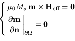 Brown's Equations