B.2 Perturbative analysis of limit cycles in 2D dynamical systems

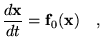
Here we present the Poincaré-Melnikov perturbative technique to analyze limit cycles in dynamical systems defined on a 2D manifold $\Sigma$. We follow the approach proposed by Perko in Ref. [43]. Let us consider an autonomous dynamical system:

$$\frac{d\textbf{x}}{dt}=\mathbf{f}_0(\textbf{x}) \quad,$$ (B.19)

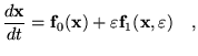
with $\textbf{x}=(x_1,x_2)\in\mathbb{R}^2$ and $\mathbf{f}_0(\textbf{x})$ analytical in $\mathbb{R}^2$. Let us suppose to perturbe the system in the following way:

$$\frac{d\textbf{x}}{dt}=\mathbf{f}_0(\textbf{x}) + \varepsilon \mathbf{f}_1(\textbf{x},\varepsilon)\quad,$$ (B.20)

where $\varepsilon$ is the amplitude of the perturbation and $\mathbf{f}_1(\textbf{x},\varepsilon)$ is an analytical function in $\mathbb{R}^2$. We assume now that the unperturbed system (B.19) has a continuous family of periodic trajectories:

$$\Gamma_{\textbf{x}_0}:\textbf{x}(t)=\gamma(\textbf{x}_0,t) \quad.$$ (B.21)

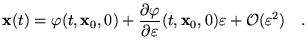
These trajectories can be determined by the initial condition $\textbf{x}_0$ chosen on a Poincaré section $S$ (see Fig. B.1 and Ref. [43]) normal to the family of periodic trajectories. Conversely, the generic trajectory of the perturbed system (B.20) will be, in general

$$\textbf{x}(t)=\varphi(t,\textbf{x}_0,\varepsilon) \quad,$$ (B.22)

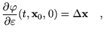
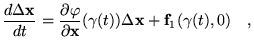
where we have indicated with $\varphi(t,\textbf{x}_0,\varepsilon)$ the flow of the dynamical system (B.20) From Eq. (B.22) it follows that:

$$\gamma(t)=\varphi(t,\textbf{x}_0,\varepsilon=0) \quad,$$ (B.23)

where, for sake of brevity, the dependance on $\textbf{x}_0$ has been not indicated. The flow (B.22) can be developed in Taylor series with respect to the perturbation parameter $\varepsilon$:

$$\textbf{x}(t)=\varphi(t,\textbf{x}_0,0)+\frac{\partial \varphi}{\... ...al \varepsilon}(t,\textbf{x}_0,0)\varepsilon+\mathcal{O}(\varepsilon^2) \quad.$$ (B.24)

By remembering Eq. (B.23) and by setting

$$\frac{\partial \varphi}{\partial \varepsilon}(t,\textbf{x}_0,0)=\Delta\textbf{x}\quad,$$ (B.25)

one obtains

$$\textbf{x}(t)=\varphi(t,\textbf{x}_0,0)+\varepsilon\Delta\textbf{x}+\mathcal{O}(\varepsilon^2) \quad.$$ (B.26)

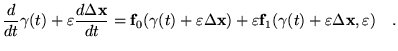
By using the latter equation in the perturbed dynamical system (B.20), we end up with:

$$\frac{d}{dt}\gamma(t)+\varepsilon\frac{d\Delta\textbf{x}}{dt}=\ma... ...repsilon\mathbf{f}_1(\gamma(t)+\varepsilon\Delta\textbf{x},\varepsilon) \quad.$$ (B.27)

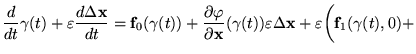
By developing in Taylor series the right-hand side of the latter equation with respect to the variables $\textbf{x},\varepsilon$, one has:

$$\frac{d}{dt}\gamma(t)+\varepsilon\frac{d\Delta\textbf{x}}{dt}=\ma... ...a(t))\varepsilon\Delta\textbf{x}+ \varepsilon \bigg(\mathbf{f}_1(\gamma(t),0)+$$

$$+\frac{\partial \mathbf{f}_1}{\partial \textbf{x}}(\gamma(t),0)\v... ...rtial \mathbf{f}_1}{\partial \varepsilon}(\gamma(t),0)\varepsilon)\bigg) \quad.$$ (B.28)

By remembering that $\frac{d}{dt}\gamma(t)=\mathbf{f}_0(\gamma(t))$ and by neglecting second order terms, one ends up with the following equation:

$$\frac{d\Delta\textbf{x}}{dt}=\frac{\partial \varphi}{\partial \textbf{x}}(\gamma(t))\Delta\textbf{x}+ \mathbf{f}_1(\gamma(t),0) \quad,$$ (B.29)

which we call first variational equation with respect to $\varepsilon$. Equation (B.29) defines a 2D dynamical system which can be used, in principle to study how the perturbation affects the displacement $\Delta\textbf{x}$ of the perturbed trajectory with respect to the unperturbed orbit in one period. We notice that the dynamical system (B.29) has periodic coefficients and, therefore it is not possible to solve it in exact analytical form.

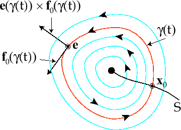
Figure: Planar sketch of a portion of the phase portrait of the unperturbed dynamical system (B.19). $S$ is the Poincaré section normal to the family of continuous trajectories.

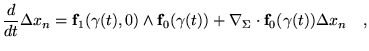
Nevertheless, we observe that we are interested only on the component of $\Delta\textbf{x}$ normal to the unperturbed trajectory $\gamma(t)$:

$$\Delta x_n=\Delta\textbf{x}\cdot \textbf{n}\quad,$$ (B.30)

where $\textbf{n}$ is the unit-vector normal to $\gamma(t)$ and tangential to the manifold $\Sigma$. The unit-vector $\textbf{n}$ is proportional to the following vector:

$$\mathbf{f}_0(\gamma(t))\times\mathbf{e}(\gamma(t)) \quad,$$ (B.31)

where $\mathbf{e}$ is the unit-vector normal to $\Sigma$. Therefore, we can express $\Delta x_n$ as

$$\Delta x_n=\Delta \textbf{x}\cdot \mathbf{f}_0(\gamma(t))\times\mathbf{e}(\gamma(t))=\Delta\textbf{x}\wedge \mathbf{f}_0(\gamma(t)) \quad,$$ (B.32)

where the wedge product $\textbf{v}\wedge\textbf{w}$, with $\textbf{v}=(v_1,v_2),\textbf{w}=(w_1,w_2)\in\mathbb{R}^2$, is defined as

$$\textbf{v}\wedge\textbf{w}=v_1 w_2-v_2 w_1 \quad.$$ (B.33)

By differentiating both sides of Eq. (B.32) with respect to time, remembering Eq. (B.29), and using straightforward algebra, one ends up with the following one-dimensional differential equation, with periodic coefficients, for $\Delta x_n$:

$$\frac{d}{dt}\Delta x_n=\mathbf{f}_1(\gamma(t),0)\wedge\mathbf{f}_0(\gamma(t))+\nabla_\Sigma\cdot \mathbf{f}_0(\gamma(t)) \Delta x_n \quad,$$ (B.34)

where $\nabla_\Sigma \cdot \mathbf{f}_0=$tr$\left[\frac{\partial \mathbf{f}_0}{\partial \textbf{x}}(\gamma(t))\right]$ is the divergence of the 2D vector field $\mathbf{f}_0(\gamma(t))$. It can be shown [43] that

$$\int_0^{T_{\textbf{x}_0}} \nabla_\Sigma \cdot \mathbf{f}_0(\gamma(t)) dt=0 \quad.$$ (B.35)

Equation (B.34) can be analytically integrated over one period of the unperturbed solution $T_{\textbf{x}_0}$. By taking into account the latter equation, the solution can be written as:

$$\Delta x_n(T_{\textbf{x}_0})=\int_0^{T_{\textbf{x}_0}} \exp\left[... ...eft[\mathbf{f}_1(\gamma(t),0)\wedge\mathbf{f}_0(\gamma(t)) \right] dt \quad.$$ (B.36)

In addition, if $\mathbf{f}_0(\textbf{x})$ is a conservative vector field it happens that:

$$\nabla_\Sigma\cdot\mathbf{f}_0=0 \quad.$$ (B.37)

Thus, Eq. (B.36) reduces to the following simpler form:

$$\Delta x_n(T_{\textbf{x}_0})=\int_0^{T_{\textbf{x}_0}} \mathbf{f}_1(\gamma(t),0)\wedge\mathbf{f}_0(\gamma(t)) dt \quad.$$ (B.38)

Let us suppose now that the generic unperturbed trajectory, determined by the initial condition $\textbf{x}_0$, can be univocally determined by a scalar parameter $g_0$ through a correspondence $g_0=g(\textbf{x}_0)$. From Eq. (B.36) one can define the Melnikov function $M(g_0)$:

$$M(g_0)=\int_0^{T_{g_0}} \exp\left[-\int_0^t \nabla_\Sigma \cdot ... ...eft[\mathbf{f}_1(\gamma(t),0)\wedge\mathbf{f}_0(\gamma(t)) \right] dt \quad,$$ (B.39)

where $T_{g_0}=T_{g(\textbf{x}_0)}$. Therefore, to summarize, the Melnikov function, computed on the value $g_0$, determines the one period displacement of the unperturbed trajectory, determined by $g_0$, in the direction normal to that unperturbed trajectory. Intuitively, it can be inferred that when $M(g_0)=0$, the unperturbed trajectory corresponding to $g_0$ becomes a limit cycle when the perturbation is introduced. This can be rigorously proven (see Ref. [43]) for finite (but small) values of the perturbation parameter $\varepsilon$. Thus, the zeros of the Melnikov function correspond to limit cycles of the perturbed dynamical system (B.20). Moreover, the sign of the derivative of the Melnikov function at the zero determines the stability of the corresponding limit cycle. In particular, positive derivative implies that the limit cycle is stable, whereas negative sign corresponds to an unstable limit cycle. By using this technique, also bifurcations of limit cycles can be studied. In particular, it is possible to find algebraic conditions which corresponds to suitable bifurcation conditions [43]. For instance, the condition for the Andronov-Hopf bifurcation is given by:

$$M(g_0)=0 \quad,\quad \frac{dM}{d g_0}=0 \quad,$$ (B.40)

and the condition for homoclinic connection bifurcation is obtained by imposing that the Melnikov function vanishes in correspondence of an unperturbed homoclinic trajectory.